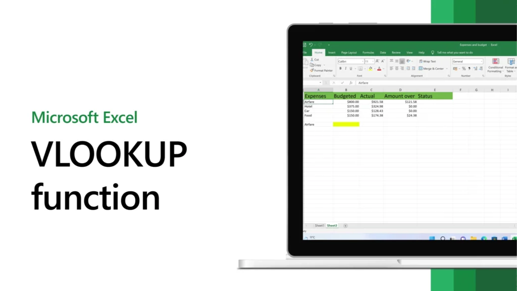
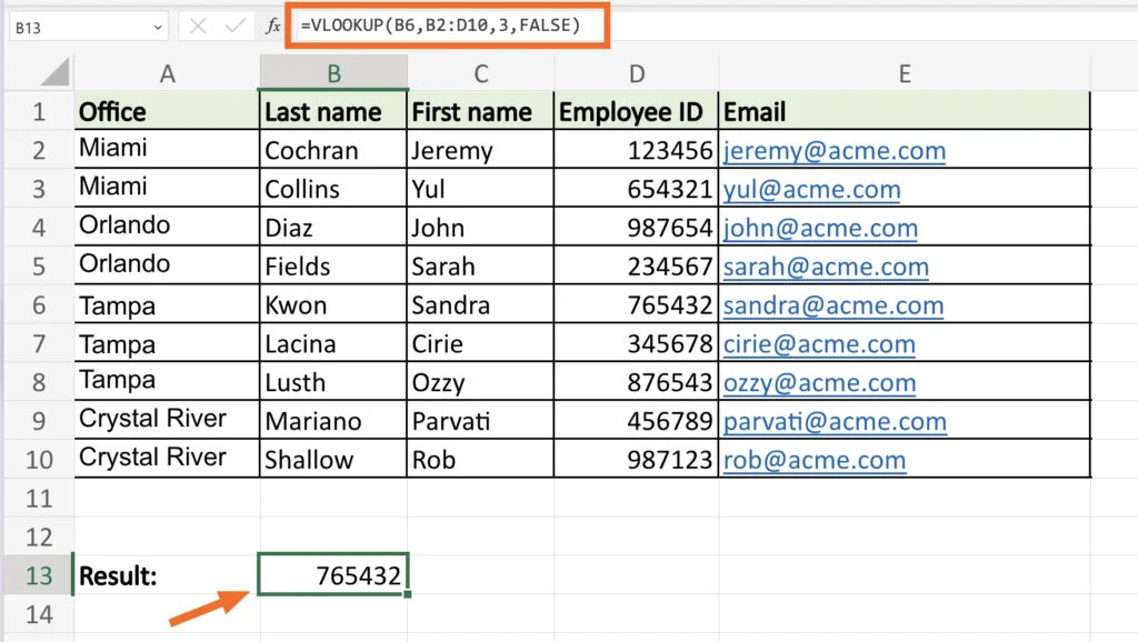
In the dynamic world of spreadsheets, Excel course for beginner stands as a powerhouse, offering a myriad of functions to manipulate and analyze data with precision and efficiency. Among these functions, VLOOKUP reigns supreme, serving as a cornerstone for data retrieval tasks. Whether you’re a seasoned Excel (Excel course for beginner) aficionado or a novice seeking to harness its capabilities, understanding how to wield the VLOOKUP function is essential for unlocking the full potential of your data analysis endeavors.
In this comprehensive guide, we’ll embark on a journey to explore the intricacies of the VLOOKUP function, unraveling its syntax, applications, and practical examples to illuminate its versatility and utility in real-world scenarios.

Understanding the Syntax of VLOOKUP
The VLOOKUP function in Excel follows a straightforward syntax:
scssCopy code
=VLOOKUP(lookup_value, table_array, col_index_num, [range_lookup])
- lookup_value: This is the value you want to search for in the first column of the table_array. It can be a specific value, cell reference, or text string.
- table_array: This is the range of cells that contains the data you want to retrieve information from. The first column of the table_array must contain the values you are searching for.
- col_index_num: This is the column number in the table_array from which you want to retrieve the data. The first column in the table_array is considered column 1.
- range_lookup: This is an optional argument that specifies whether you want an exact match (FALSE) or an approximate match (TRUE or omitted). If omitted, VLOOKUP defaults to an approximate match.

Retrieving Data from a Table
Let’s delve into a simple example to illustrate the basic usage of the VLOOKUP function. Suppose we have a dataset containing employee information, and we want to retrieve the department of an employee based on their employee ID.
excelCopy code
=VLOOKUP(A2, EmployeeData, 2, FALSE)
In this formula:
- A2 represents the cell containing the employee ID we want to look up.
- EmployeeData is the range of cells containing the employee data, with the department information located in the second column.
- We specify 2 as the col_index_num to retrieve data from the second column (department).
- By setting range_lookup to FALSE, we ensure that VLOOKUP performs an exact match.

Handling Missing Values with VLOOKUP
One of the key advantages of the VLOOKUP function is its ability to handle missing or unknown values gracefully. Suppose we have a dataset containing product information, and we want to retrieve the price of a product based on its product code. If the product code is not found in the dataset, we want Excel to display “Not Found” instead of an error.
excelCopy code
=IFERROR(VLOOKUP(B2, ProductData, 2, FALSE), "Not Found")
In this enhanced formula:
- B2 represents the cell containing the product code we want to look up.
- ProductData is the range of cells containing the product data, with the price information located in the second column.
- We use the IFERROR function to handle errors gracefully. If VLOOKUP encounters an error (e.g., the product code is not found), it returns “Not Found” instead of displaying an error message.
Leveraging VLOOKUP with Named Ranges
Named ranges offer a convenient way to enhance the readability and usability of your formulas in Excel (Excel course for beginner). By assigning descriptive names to ranges of cells, you can streamline your formulas and make them easier to understand and maintain. Let’s consider an example where we have a named range called “EmployeeID” for the employee IDs and a named range called “EmployeeDepartment” for the corresponding departments.
excelCopy code
=VLOOKUP(A2, EmployeeID:EmployeeDepartment, 2, FALSE)
In this refined formula:
- EmployeeID:EmployeeDepartment represents the named range spanning from the EmployeeID range to the EmployeeDepartment range.
- By using named ranges, we enhance the clarity and readability of the formula, making it easier to understand and manage.
Advanced Applications of VLOOKUP
The VLOOKUP function can be customized and extended to handle more complex data retrieval tasks. By combining it with other Excel functions and techniques, you can unlock a world of possibilities for data analysis and decision-making. Some advanced applications of VLOOKUP include:
- Using wildcard characters to perform partial matches.
- Employing nested functions to handle multi-level lookups.
- Dynamically updating table references using structured references.
Conclusion
In conclusion, the VLOOKUP function stands as a formidable ally in the arsenal of Excel users (Excel course for beginner), empowering them to retrieve data from tables with precision and efficiency. From basic data lookup tasks to advanced applications, its versatility and flexibility make it indispensable for a wide range of data analysis and decision-making scenarios.
By mastering the syntax and applications of the VLOOKUP function, you can streamline your data retrieval processes, enhance the accuracy of your analyses, and unlock new insights hidden within your datasets. Experiment with different scenarios, explore advanced functionalities, and embrace the transformative potential of VLOOKUP in shaping your Excel journey.
As you embark on your exploration of Excel’s vast capabilities, let VLOOKUP be your trusted companion in navigating the seas of data, guiding you towards informed decisions and data-driven insights that propel your success in the world of spreadsheets.


