Working with data in Excel often means you need to look up a value that doesn’t exactly exist but falls within a range. That’s where approximate match lookups come in handy. Using INDEX MATCH and match_type in Excel, you can build reliable and flexible formulas. By combining INDEX in Excel with MATCH in Excel and correctly setting the match_type in Excel, you gain precise control over range-based lookups—an essential skill when learning Excel basic and advanced techniques.
In this tutorial, you’ll learn how to perform powerful lookups for grading systems, tax brackets, and commission rates using INDEX MATCH and match_type in Excel, combining INDEX in Excel and MATCH in Excel with the correct match_type in Excel—a practical skill taught in Excel basic and advanced learning.
🧠 What is an Approximate Match?
An approximate match finds the closest value without going over, based on a sorted list.
- Grades: Score of 88 = “B+” (Range 80–89)
- Tax: Income of $45,000 matches the 40k bracket
- Shipping: Weight of 2.3 kg falls in the 2–3kg category

🔍 What are INDEX and MATCH?
✅ INDEX Function
Returns the value at a specific position.
=INDEX(array, row_num, [col])✅ MATCH Function
Returns position. match_type controls the logic:
- 1: Less than or equal to (Ascending)
- 0: Exact match
- -1: Greater than or equal to (Descending)
🧪 Real-Life Example: Grading System
Imagine a student scoring 78 and you want to assign a grade based on this grading scale:
| Minimum Score | Grade |
| 0 | F |
| 50 | D |
| 60 | C |
| 70 | B |
| 80 | A |
| 90 | A+ |
This is a perfect use case for approximate match lookups.
✅ Step 1: Structure Your Data
Create the grade table in cells A2:B7:
| A | B |
|---|---|
| 0 | F |
| 50 | D |
| 60 | C |
| 70 | B |
| 80 | A |
| 90 | A+ |
Enter the student’s score in cell D2.
✅ Step 2: Write the INDEX MATCH Formula
=INDEX(B2:B7, MATCH(D2, A2:A7, 1))🔍 How It Works:
- MATCH(D2, A2:A7, 1) searches for the highest score less than or equal to the student’s score
- INDEX(B2:B7, …) returns the grade at that position
If D2 = 78, MATCH finds 70 → row 4 → returns B
If D2 = 85, MATCH finds 80 → row 5 → returns A
This is how you perform approximate match using INDEX and MATCH with match_type = 1.
📘 Why match_type = 1?
The match_type controls how Excel searches:
- 1 → finds the largest value less than or equal to your lookup value (requires list sorted in ascending order)
- 0 → exact match only
- -1 → finds the smallest value greater than or equal to (list must be in descending order)
So when using range-based data like grading, taxes, or thresholds, match_type = 1 is perfect.
🔧 Example 2: Tax Bracket Lookup
| Income Threshold | Tax Rate |
| 0 | 10% |
| 10000 | 15% |
| 30000 | 20% |
| 60000 | 25% |
| 100000 | 30% |
Find rate for $45,000:
=INDEX(B2:B6, MATCH(45000, A2:A6, 1))Result: 20% (45k is between 30k and 60k)
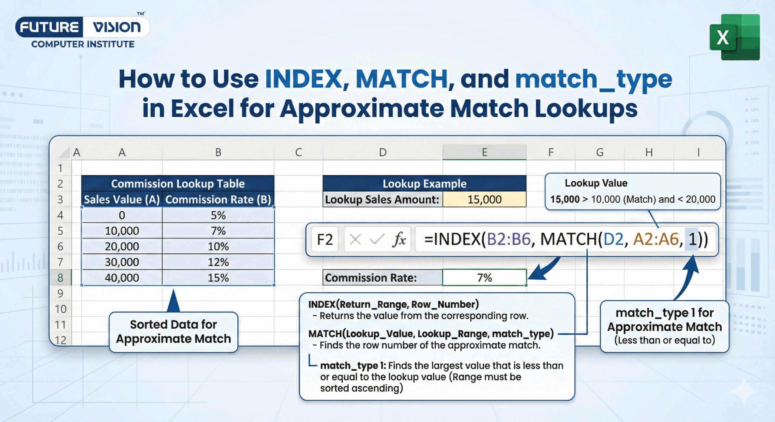
📈 Example 3: Commission Rate Table
| Sales Threshold | Commission % |
| 0 | 2% |
| 1000 | 4% |
| 5000 | 6% |
| 10000 | 8% |
| 20000 | 10% |
Sales rep closed $12,500 in sales.
Formula:
=INDEX(B2:B6, MATCH(12500, A2:A6, 1))Result: 8%
Because 12500 is greater than 10000 but less than 20000.
🛠 Bonus: Create a Dynamic Lookup with a Cell Reference
Instead of hardcoding the lookup value (e.g. 45000), let users input it in a cell, say D2.
=INDEX(B2:B6, MATCH(D2, A2:A6, 1))This way, your formula becomes dynamic—changing D2 automatically updates the result.
🧠 Pro Tips for INDEX MATCH Approximate Lookups
✅ 1. Use match_type = 1 for thresholds
It gives you the “greatest value less than or equal to” logic that range-based systems need.
✅ 2. Sort the lookup column in ascending order
Your lookup array (the first parameter in MATCH) must be sorted. If not, the formula can return incorrect results.
✅ 3. Use named ranges for better readability
For example:
=INDEX(GradeList, MATCH(StudentScore, ScoreThreshold, 1))✅ 4. Combine with IFERROR() for user-friendly messages
=IFERROR(INDEX(B2:B6, MATCH(D2, A2:A6, 1)), "Not in range")🚫 Common Errors to Avoid
| Mistake | Why It’s a Problem |
| Using match_type 1 with unsorted data | Returns wrong or misleading values |
| Forgetting to match INDEX’s array with MATCH’s result | INDEX row must match MATCH position |
| Using match_type = 0 when value doesn’t exist | Returns #N/A |
| Mixing up ascending and descending rules | match_type = 1 is for ascending; -1 for descending only |
📘 TL;DR – Master Formula
=INDEX(ResultRange, MATCH(LookupValue, ThresholdRange, 1))Used when:
- Your data is based on ranges or thresholds
- You want to return a result based on the closest lower match
- Your values are sorted in ascending order
✅ Final Thoughts
Using INDEX, MATCH, and the match_type parameter in Excel allows you to build smart, dynamic formulas for approximate match lookups—the kind used in grading scales, tax brackets, commission tables, and pricing thresholds. Mastering this technique is a key part of Excel basic and advanced learning for real-world data analysis.
Once you understand the match_type parameter:
- 1 for approximate match in ascending order
- 0 for exact match
- -1 for descending lookups
…you’ll unlock Excel’s full lookup power.
Whether you’re building dashboards, automating reports, or analyzing financial data, this formula combo gives you the speed, accuracy, and flexibility your spreadsheets need—an essential skill when mastering Excel basic and advanced workflows.
🔗 What’s Next?
- Learn how to do two-way lookups with INDEX(MATCH(…), MATCH(…))
- Combine IF, INDEX, and MATCH for advanced logic
Explore XLOOKUP (modern Excel alternative with built-in approximate match)
Find Our Locations
Visit any of our three convenient branches or contact us directly.
Pal Branch
Address: 115, Raj Victoria Complex, Pal Gam Circle, Pal.
Phone: +91-9825771641
Unlock Excel’s Full Potential
Whether for grading, taxes, or commissions, approximate matches are a powerful tool for your Excel toolbox.