If you’re an Excel user, you’ve probably heard of VLOOKUP, maybe even INDEX and MATCH in Excel, but what happens when you need to look up a value based on both a row and a column label? That’s where a two-way lookup comes in. By combining INDEX in Excel with MATCH in Excel, you can perform powerful matrix lookups used in real-world reporting and dashboards. These skills are essential for learners progressing from basic Excel and advanced Excel levels and are commonly taught at an advanced Excel course institute near me to build strong data analysis expertise.

The best tool for this is a powerful combo of INDEX (to retrieve a value), MATCH (to find the row), and another MATCH (to find the column). Let’s break down exactly how to build this dynamic formula — a core skill taught at an advanced Excel course institute near me for real-world data analysis.

🧠 What is a Two-Way Lookup?

A two-way lookup searches for a value based on both a row heading and a column heading. Think of it as looking up data in a grid, where both the row and column matter.

📊 Example Scenario:

You manage monthly sales data for multiple products:

	Jan	Feb	Mar
Apple	100	120	140
Banana	80	90	95
Mango	110	130	125

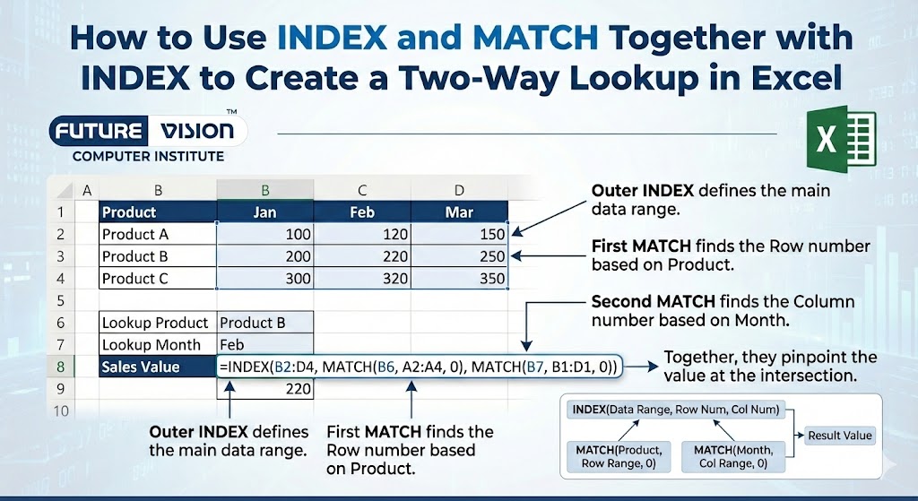
The Core Formula:

=INDEX(data_range, MATCH(row_val, row_headers, 0), MATCH(col_val, col_headers, 0))

• Second MATCH finds the Column Number.
• First MATCH finds the Row Number.

✅ Step-by-Step Example: Monthly Sales Lookup

Organize Your Data

	A	B	C	D
	Jan	Feb	Mar
Apple	100	120	140
Banana	80	90	95
Mango	110	130	125

• Row headers: A3:A5
• Column headers: B2:D2
• Data grid: B3:D5

Set Up Lookup Values

• In F2: Product name (e.g. Banana)
• In F3: Month name (e.g. Feb)

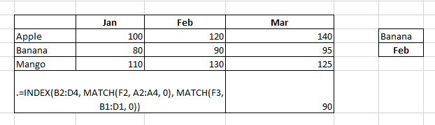
Build the Formula

=INDEX(B3:D5, MATCH(F2, A3:A5, 0), MATCH(F3, B2:D2, 0))

✅ How it works:

• MATCH(F2, A3:A5, 0) → finds the row position for Banana → returns 2
• MATCH(F3, B2:D2, 0) → finds column position for Feb → returns 2
• INDEX(B3:D5, 2, 2) → returns 90 (sales of Banana in Feb)

This is your two-way lookup formula in Excel—it dynamically returns a value based on two input conditions.

🧪 Real-Life Example: Employee Hours

	Mon	Tue	Wed
John	8	9	7
Sarah	6	8	10
Dave	7	6	9

Want to know how many hours Sarah worked on Wednesday?

=INDEX(B2:D4, MATCH("Sarah", A2:A4, 0), MATCH("Wed", B1:D1, 0))

Result: 10.

💡 Why Use INDEX + MATCH Instead of VLOOKUP or HLOOKUP?

Feature	VLOOKUP / HLOOKUP	INDEX + MATCH
Can look left or up	❌	✅
Requires exact column/row #	✅ (static)	✅ (but dynamic with MATCH)
Works in two directions	❌	✅
Breaks when columns change	✅ Yes	❌ No
Dynamic and flexible	❌	✅

This is why INDEX MATCH MATCH is preferred for professional-grade spreadsheets and dashboards.

🔄 Make the Formula Dynamic with Cell References

Instead of hardcoding “Sarah” and “Wed”, use:

• F2: employee name
• F3: weekday

=INDEX(B2:D4, MATCH(F2, A2:A4, 0), MATCH(F3, B1:D1, 0))

Now, change values in F2 or F3, and your formula instantly shows the matching result. This makes it perfect for dynamic reports or dashboards.

🧠 Pro Tips for Two-Way Lookups in Excel

1. Always use match_type = 0 in MATCH

This forces exact match, which is safer and more predictable than approximate matching.

MATCH("Feb", B2:D2, 0)

2. Use named ranges

Instead of writing A3:A5, name it ProductList, and your formula becomes:

=INDEX(SalesData, MATCH(F2, ProductList, 0), MATCH(F3, MonthList, 0))

This improves readability and reduces errors.

3. Add IFERROR for cleaner outputs

=IFERROR(INDEX(B3:D5, MATCH(F2, A3:A5, 0), MATCH(F3, B2:D2, 0)), "Not found")

This prevents errors like #N/A from breaking your dashboard.

📘 Advanced Variation: Case-Insensitive Two-Way Lookup

Excel’s MATCH is not case-sensitive. If you want to ensure cleaner logic, wrap your MATCH inputs with UPPER() or LOWER():

=MATCH(UPPER(F2), UPPER(A3:A5), 0)

Just make sure all your data is in consistent case format.

🛠 Bonus Example: Cross-Reference Cost Table

	Basic	Premium	Enterprise
Email	10	15	25
Hosting	50	70	100
Support	20	30	50

=INDEX(B2:D4, MATCH(“Hosting”, A2:A4, 0), MATCH(“Premium”, B1:D1, 0))

Returns: 70

🚫 Common Mistakes to Avoid

Mistake	Why it’s a problem
Using approximate match by default	Leads to wrong results—always use 0 in MATCH
Misaligning INDEX and MATCH ranges	MATCH must correspond exactly to INDEX ranges
Including headers in INDEX array	Will return the wrong row/column
Not anchoring references properly	Causes errors when dragging formulas

📘 TL;DR – Master Two-Way Lookup Formula

=INDEX(data_range, MATCH(row_value, row_labels, 0), MATCH(column_value, column_labels, 0))

✅ Final Thoughts

Learning how to create a two-way lookup using INDEX and MATCH in Excel gives you a powerful edge in data analysis, reporting, and dashboard creation — exactly the kind of skill taught at an advanced Excel course institute near me.

You now know how to:

• Create flexible lookups across both rows and columns
• Dynamically return results based on user input
• Avoid the limitations of VLOOKUP and HLOOKUP

This technique is foundational for anyone building clean, professional, and scalable Excel solutions.

Find Our Locations

Visit any of our three convenient branches or contact us directly.

Turn Negatives Into Productivity!

Master functions like ABS, MOD, and Pivot Tables with our specialized

courses in Advanced Excel and Data Science.