If you’ve worked in Excel for more than five minutes, you’ve probably used VLOOKUP in Excel. It’s easy, popular, and useful—but what happens when your data structure isn’t “VLOOKUP-friendly”? That’s where INDEX in Excel and MATCH in Excel step in. Together, VLOOKUP, INDEX and MATCH in Excel create a supercharged, flexible, and dynamic lookup solution that outperforms traditional lookups in nearly every way. Mastering these formulas is a key part of advanced Excel and Power BI, helping you build smarter, more powerful data analysis models.
In this post, we’ll walk you through how to use VLOOKUP, INDEX, and MATCH together. We’ll make it simple, practical, and easy to understand—even if you’re just starting out.
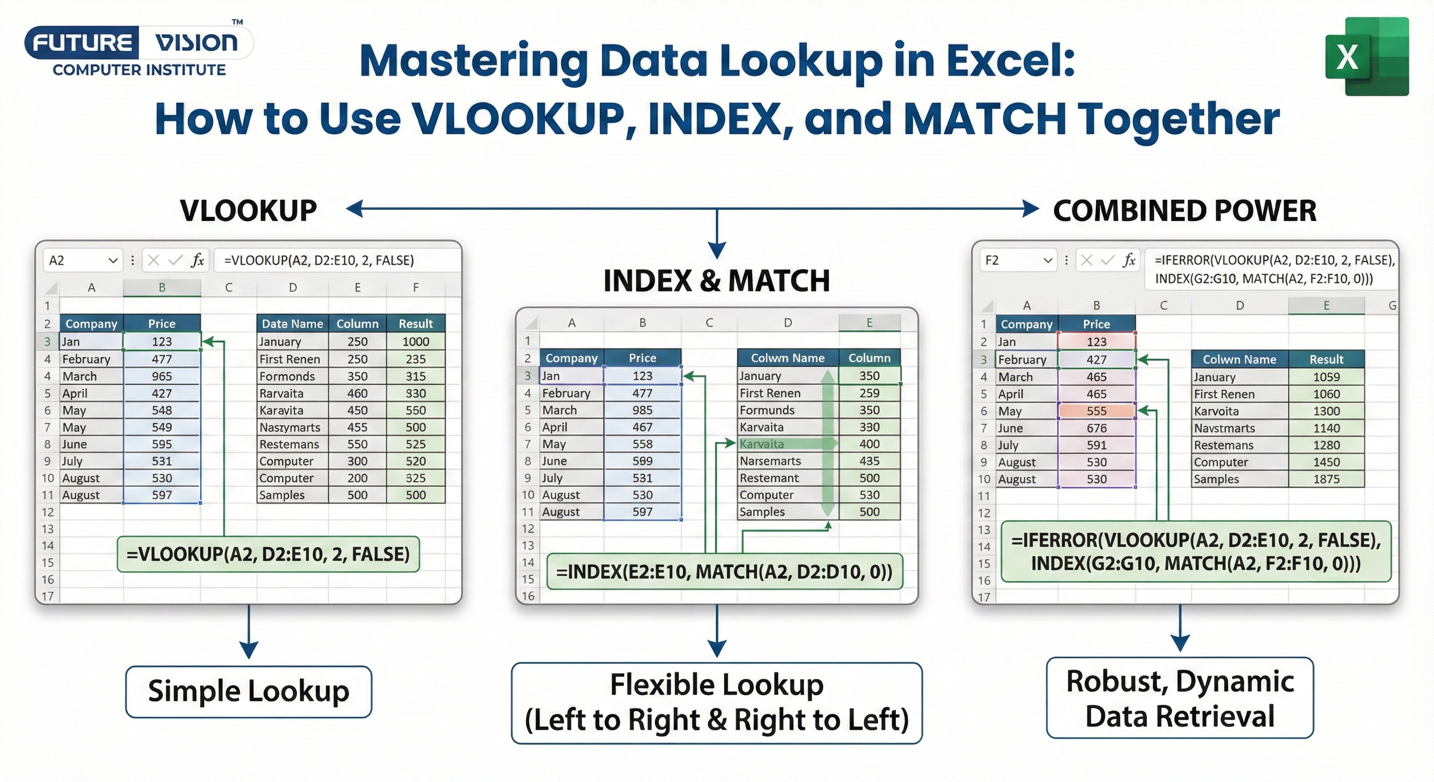
🧩 Why Combine VLOOKUP, INDEX, and MATCH?
✅ VLOOKUP
Searches vertical list.
=VLOOKUP(lookup_value, table, col_index, [range])✅ INDEX
Returns value at position.
=INDEX(array, row_num, [col_num])✅ MATCH
Returns position of value.
=MATCH(lookup_value, array, [type])🚫 The Problem with VLOOKUP Alone
- It only searches left to right.
- It breaks if the column order changes.
- It’s hard-coded, so it’s not dynamic.
That’s why we combine it with INDEX and MATCH—for flexibility, accuracy, and power.
🧠 Real-Life Example: Employee Salary Lookup
Scenario: You have a list of employees, their departments, and their salaries. You want to search for a name and department and return their salary—dynamically.
| Employee | Department | Salary |
| John | Sales | 50000 |
| Sarah | HR | 60000 |
| Alex | IT | 55000 |
| John | IT | 58000 |
| Sarah | Sales | 62000 |
Now, you want to create a formula where:
- You enter Employee Name and Department in input cells.
- Excel returns the correct Salary, even if there are duplicates.
✍️ Step-by-Step: Using INDEX + MATCH for Two Conditions
🎯 Step 1: Combine Name and Department Columns (Helper Column)
In a new column (say Column D), combine Employee and Department:
=A2 & "-" & B2Now Column D looks like:
| Employee-Department |
| John-Sales |
| Sarah-HR |
| Alex-IT |
| John-IT |
| Sarah-Sales |
🎯 Step 2: Create Dynamic Input Fields
In another part of the sheet:
| Cell | Purpose |
| F2 | Employee Name |
| G2 | Department |
| H2 | Combined Lookup Key = =F2 & “-” & G2 |
🎯 Step 3: Use INDEX + MATCH
Now, use this formula in I2 to get the salary:
=INDEX(C2:C6, MATCH(H2, D2:D6, 0))Explanation:
- MATCH(H2, D2:D6, 0) → finds the row number where the name+department match.
- INDEX(C2:C6, …) → pulls the salary from that row.
Boom. 🔥 Dynamic lookup based on two conditions—without relying on complex nested IFs or error-prone VLOOKUPs.
🧬 What About Using VLOOKUP + MATCH?
Instead of hardcoding the column index (e.g., “3” for Salary), use MATCH to find the column number dynamically. This prevents errors if you insert new columns later.
| Employee | Department | Salary | Bonus |
| John | Sales | 50000 | 5000 |
| Sarah | HR | 60000 | 6000 |
| Alex | IT | 55000 | 5500 |
=VLOOKUP("Alex", A2:D4, MATCH("Bonus", A1:D1, 0), FALSE)Explanation:
- MATCH(“Bonus”, A1:D1, 0) returns column number of “Bonus” (which is 4).
- Now VLOOKUP dynamically adjusts if columns are reordered.

💡 Pro Tips for Lookup Formulas
1. Use Named Ranges:
Instead of A2:A10, use EmployeeList—makes your formulas readable.
2. Use Tables:
Convert data to Excel Table (Ctrl + T) and use structured references.
Example:
=INDEX(Table1[Salary], MATCH(H2, Table1[Key], 0))3. Combine IFERROR:
To hide #N/A errors:
=IFERROR(INDEX(...), "Not found")🛠 Advanced: INDEX MATCH MATCH (Two-Way Lookup)
Want to look up a value based on both a specific row (Name) and a specific column (Month)? It’s like a 2D VLOOKUP.
| Jan | Feb | Mar | |
| John | 500 | 550 | 530 |
| Sarah | 600 | 580 | 590 |
=INDEX(B2:D3, MATCH("Sarah", A2:A3, 0), MATCH("Feb", B1:D1, 0))It’s like a two-dimensional VLOOKUP.
🔐 Why INDEX + MATCH is Better Than VLOOKUP
If someone’s Googling “VLOOKUP vs INDEX MATCH”, this is what they need to hear:
| Feature | VLOOKUP | INDEX + MATCH |
| Left Lookup | ❌ No | ✅ Yes |
| Dynamic Column Ref | ❌ Hardcoded | ✅ MATCH makes it dynamic |
| Column Insert Safe | ❌ Breaks easily | ✅ Flexible |
| Speed on Big Data | ❌ Slower | ✅ Faster |
| Multi-condition | ❌ Not native | ✅ Easily doable |
🔄 Dynamic Drop-downs With Lookup (Bonus Tip)
Want users to select a name and department from a drop-down?
- Create Data Validation for Employee (F2) and Department (G2).
- Let Excel auto-populate Salary based on the dynamic formula.
This makes your dashboard cleaner, error-proof, and user-friendly.
🧠 TL;DR – Final Formula Breakdown
- Basic Lookup (VLOOKUP):
=VLOOKUP("John", A2:C6, 3, FALSE)- Dynamic Column VLOOKUP:
=VLOOKUP("Alex", A2:D4, MATCH("Bonus", A1:D1, 0), FALSE)- Two Criteria (INDEX + MATCH):
=INDEX(C2:C6, MATCH(F2 & "-" & G2, D2:D6, 0))📌 Final Thoughts
Excel’s true power lies in its ability to adapt and respond to data dynamically, and nothing shows that better than combining VLOOKUP, INDEX, and MATCH. While VLOOKUP is a great starter tool, INDEX + MATCH gives you flexibility, performance, and control—all essential in real-world spreadsheet scenarios.
So next time you’re building a report or dashboard, skip the basic VLOOKUP and elevate your game with these robust lookup formulas.
Want to Go Even Further?
- Learn about XLOOKUP – the modern replacement of VLOOKUP (coming soon!)
- Automate reports with dynamic named ranges and OFFSET functions.
- Use Power Query to merge and clean data before using lookup formulas.
If you found this guide helpful, save it, share it, and stay tuned for more Excel ninja tricks!
Would you like me to optimize this entire blog post to hit 100/100 in Rank Math Pro? That includes:
- SEO title
- Slug
- Meta description
- OG image and schema
- Focus keywords and placement
Just say the word, and I’ll get it SEO-polished to perfection.